
Ping Pong Buffers
As Andrei described DMA theory and two examples of implementation, I kept wondering when he’d write about using it the way I often do: a slow peripheral trickling in data until there is enough to run some algorithm on. (To be fair, Andrei kept wondering when I’d write the post about ping pong buffers I’d promised and forgotten about.)
Using ping pong buffers is not a difficult concept, it is just a way of moving memory back and forth so that different parts of the system can use it without colliding. See system architecture below.
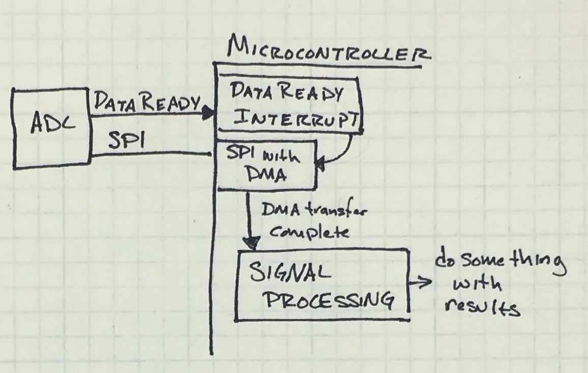
Sketch of system under discussion.
Say you have an external, high-precision ADC attached to the SPI bus, sampling at 96kHz, maybe for an audio widget. The ADC needs its buffer read to avoid losing data but the process is simple:
Processor receives DataReady interrupt.
Using DMA, the SPI sends the ADC read command and enough 0xFF dummy bytes to transfer one sample.
As the DataReady GPIO interrupt kicks off a DMA-based SPI transfer, the main loop of the processor never needs to know any of this happened. In fact, you could do this a few hundred times until you had enough samples to actually do something with data: run through signal processing, compress, and/or store to some memory (like an SD card).
With that in mind, the data acquisition process becomes:
Processor receives DataReady interrupt.
Using DMA, the SPI sends the ADC read command and enough 0xFF dummy bytes to transfer one sample.
Repeat steps 1 and 2 until buffer of N samples is full, causing the DMAComplete interrupt.
DMAComplete interrupt: signal algorithm to run.
(Non-interrupt) Algorithm runs on data.
The first four steps happen very quickly, mostly in the hardware so they don’t take many processor cycles. This leaves us more time to do that last step, the fun part of turning raw data into actionable intelligence. Let’s look at how these interrupts would happen in time.
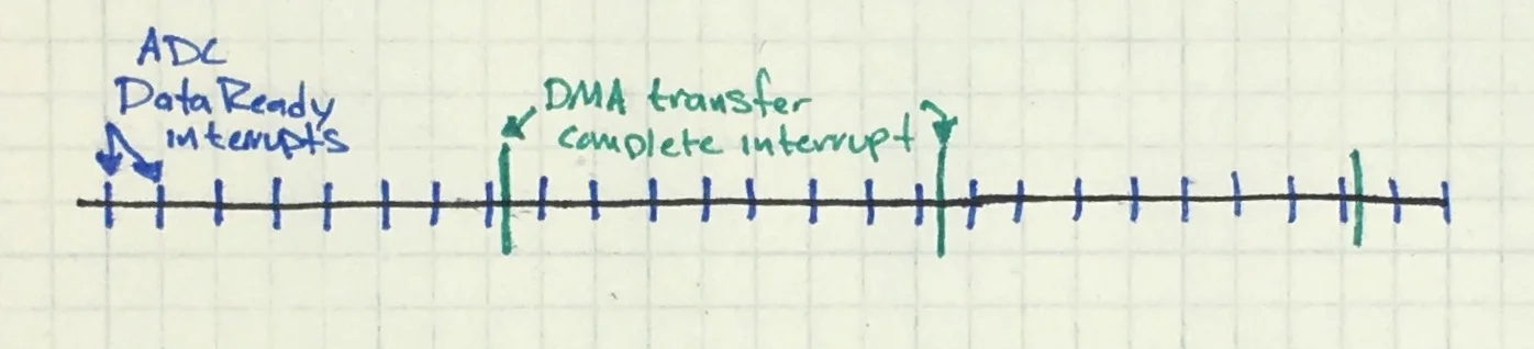
Timeline showing periodic ADC reads followed by a DMA complete interrupt after N samples (N=8 in image).
Imagine a buffer filling up with ADC samples. A problem happens when there is only one sample between when the DMAComplete interrupt the new ADC sample. As soon as the next ADC sample is ready, it goes into your buffer, the one you are currently doing algorithmic magic on. You could copy the whole thing out, but that is a waste of cycles.
Instead, we can use a ping pong buffer. Allocate two buffers of size N (the number of samples you need for the algorithm). We’ll call one Ping and the other Pong.
We will change the SPI/DMA initialization code to store the SPI data into the Ping buffer. Then, in the DMAComplete interrupt, you’d do something like:
    If the currently-in-use-buffer is Ping:
        Set DMA currently-in-use buffer to use Pong
        Signal runtime to process Ping
    Else(currently-in-use-buffer is Pong):
        Set DMA currently-in-use buffer to use Ping
        Signal runtime to process Pong
The system flips back and forth between the buffers, letting you run the algorithm on one buffer, then the other, back and forth until the end of time.
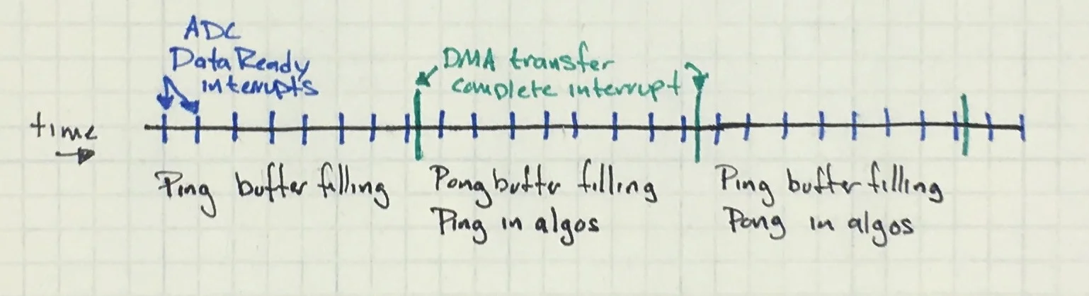
Timeline showing periodic ADC interrupts and current status of the ping pong buffers.
If you are thinking that this is a lot like a 2-element circular buffer, you are entirely correct. Thus, if your processing takes longer than the data collection time, go for a circular buffer (of buffers). This gets a little mentally complicated but a drawing of what you want will help immensely.
Note: ping pong buffers are not a new concept. I’ve used it for audio and other data processing a few times. You often see it used in sending data to displays as well as working on video input where it is usually called double buffering.